Step-by-Step Tutorial to Build a GAN from Scratch

Introduction

Generative Adversarial Networks (GANs) have transformed the landscape of artificial intelligence by enabling machines to generate data that resembles real-world examples. Introduced by Ian Goodfellow in 2014, GANs consist of two neural networks—the generator and the discriminator—that compete against each other in a zero-sum game. This tutorial will guide you through building a GAN from scratch using Python and TensorFlow/Keras, providing detailed explanations at each step. Whether you’re a beginner or an expert, this step-by-step guide is designed to be engaging and informative.

1. Understanding GANs

1.1 What Are Generative Adversarial Networks?

Generative Adversarial Networks are a class of machine learning frameworks where two models are trained simultaneously:

• Generator (G): Learns to generate new data that resembles the real data.
• Discriminator (D): Learns to distinguish between real data and data produced by the generator.

For more on how AI can generate content and learn complex tasks, explore our guide to reinforcement learning.

1.2 How GANs Work

The generator and discriminator engage in a minimax game:

• Generator’s Goal: Produce data that is so realistic that the discriminator cannot tell it apart from real data.
• Discriminator’s Goal: Accurately distinguish between real data and fake data generated by the generator.

This adversarial process continues until the discriminator cannot reliably distinguish between real and generated data.

1.3 Applications of GANs

• Image Generation: Creating realistic images, including faces, objects, and scenes.
• Data Augmentation: Enhancing datasets for training machine learning models.
• Style Transfer: Applying artistic styles to images.
• Super-Resolution: Enhancing the resolution of images.
• Anomaly Detection: Identifying unusual patterns in data.

---

2. Prerequisites

2.1 Skills and Knowledge Required

• Python Programming: Basic to intermediate level.
• Machine Learning Concepts: Understanding of neural networks and deep learning.
• Mathematics: Familiarity with linear algebra and probability is helpful.

2.2 Setting Up the Environment

Ensure you have the following installed:

• Python 3.6 or higher
• TensorFlow 2.x
• NumPy
• Matplotlib

You can install the required libraries using pip:

bash
pip install tensorflow numpy matplotlib

3. Data Preparation

3.1 Choosing the Dataset

We’ll use the MNIST dataset, which consists of 70,000 grayscale images of handwritten digits (28×28 pixels). It’s a great starting point for experimenting with GANs.

3.2 Preprocessing the Data

python
import tensorflow as tf
import numpy as np

# Load the dataset
(x_train, _), (_, _) = tf.keras.datasets.mnist.load_data()

# Normalize the images to [-1, 1]
x_train = x_train.astype('float32')
x_train = (x_train - 127.5) / 127.5

# Reshape the data to include the channel dimension
x_train = x_train.reshape(x_train.shape[0], 28, 28, 1)

4. Building the Generator Network

4.1 Understanding the Generator Architecture

The generator takes random noise as input and produces an image. We’ll use:

• Dense Layers: To transform the input noise into a meaningful representation.
• LeakyReLU Activation: To allow gradients to flow through for negative inputs.
• Batch Normalization: To stabilize and accelerate training.
• Reshape and Conv2DTranspose Layers: To upsample the data to the desired image size.

4.2 Implementing the Generator in Code

python
from tensorflow.keras.layers import Dense, Reshape, BatchNormalization, LeakyReLU, Conv2DTranspose
from tensorflow.keras.models import Sequential

def build_generator():
    model = Sequential()

    # Input layer
    model.add(Dense(7 * 7 * 256, input_dim=100))
    model.add(LeakyReLU(alpha=0.2))
    model.add(Reshape((7, 7, 256)))

    # First upsampling layer
    model.add(Conv2DTranspose(128, kernel_size=5, strides=1, padding='same'))
    model.add(BatchNormalization())
    model.add(LeakyReLU(alpha=0.2))

    # Second upsampling layer
    model.add(Conv2DTranspose(64, kernel_size=5, strides=2, padding='same'))
    model.add(BatchNormalization())
    model.add(LeakyReLU(alpha=0.2))

    # Third upsampling layer
    model.add(Conv2DTranspose(1, kernel_size=5, strides=2, padding='same', activation='tanh'))

    return model

generator = build_generator()
generator.summary()

Want to understand how neural layers, weights, and activation functions work internally? Read How Neural Networks Work.

5. Building the Discriminator Network

5.1 Understanding the Discriminator Architecture

The discriminator is a binary classifier that outputs the probability of the input image being real. We’ll use:

• Conv2D Layers: To extract features from images.
• LeakyReLU Activation: For better gradient flow.
• Dropout Layers: To prevent overfitting.
• Flatten and Dense Layers: To output a single probability value.

5.2 Implementing the Discriminator in Code

python
from tensorflow.keras.layers import Conv2D, Flatten, Dropout
from tensorflow.keras.models import Sequential

def build_discriminator():
    model = Sequential()

    # First convolutional layer
    model.add(Conv2D(64, kernel_size=5, strides=2, padding='same', input_shape=(28,28,1)))
    model.add(LeakyReLU(alpha=0.2))
    model.add(Dropout(0.3))

    # Second convolutional layer
    model.add(Conv2D(128, kernel_size=5, strides=2, padding='same'))
    model.add(LeakyReLU(alpha=0.2))
    model.add(Dropout(0.3))

    # Flatten and output layer
    model.add(Flatten())
    model.add(Dense(1, activation='sigmoid'))

    return model

discriminator = build_discriminator()
discriminator.summary()

6. Compiling the GAN

6.1 Combining the Generator and Discriminator

To train the generator, we need to combine it with the discriminator:

• Freeze the Discriminator’s Weights: So that only the generator is trained during combined model training.
• Create a Sequential Model: That feeds the generator’s output directly into the discriminator.

6.2 Defining Loss Functions and Optimizers

python
from tensorflow.keras.optimizers import Adam

# Compile the discriminator
discriminator.compile(loss='binary_crossentropy', optimizer=Adam(learning_rate=0.0002, beta_1=0.5), metrics=['accuracy'])

# Build and compile the combined model
def build_gan(generator, discriminator):
    discriminator.trainable = False
    model = Sequential()
    model.add(generator)
    model.add(discriminator)
    return model

gan = build_gan(generator, discriminator)
gan.compile(loss='binary_crossentropy', optimizer=Adam(learning_rate=0.0002, beta_1=0.5))

7. Training the GAN

7.1 The Training Loop Explained

Training a GAN involves two main steps:

1. Train the Discriminator:
   • Use a batch of real images labeled as real.
   • Generate a batch of fake images using the generator and label them as fake.
   • Update the discriminator’s weights based on the loss.
2. Train the Generator:
   • Generate a batch of noise samples.
   • Pass them through the combined model (generator + discriminator).
   • Label the outputs as real to trick the discriminator.
   • Update the generator’s weights based on the loss.

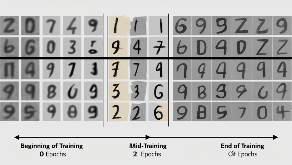
7.2 Monitoring Progress and Visualizing Results

python
import numpy as np
import matplotlib.pyplot as plt

def train(epochs, batch_size=128, save_interval=200):
    # Load and preprocess data
    X_train = x_train

    # Labels for real and fake images
    real = np.ones((batch_size, 1))
    fake = np.zeros((batch_size, 1))

    for epoch in range(epochs):

        # ---------------------
        #  Train Discriminator
        # ---------------------

        # Select a random batch of real images
        idx = np.random.randint(0, X_train.shape[0], batch_size)
        imgs = X_train[idx]

        # Generate fake images
        noise = np.random.normal(0, 1, (batch_size, 100))
        gen_imgs = generator.predict(noise)

        # Train the discriminator
        d_loss_real = discriminator.train_on_batch(imgs, real)
        d_loss_fake = discriminator.train_on_batch(gen_imgs, fake)
        d_loss = 0.5 * np.add(d_loss_real, d_loss_fake)

        # ---------------------
        #  Train Generator
        # ---------------------

        # Generate noise
        noise = np.random.normal(0, 1, (batch_size, 100))

        # Train the generator (through the combined model)
        g_loss = gan.train_on_batch(noise, real)

        # Print progress
        if epoch % save_interval == 0:
            print(f"{epoch} [D loss: {d_loss[0]:.4f}, acc.: {100*d_loss[1]:.2f}%] [G loss: {g_loss:.4f}]")
            save_images(epoch)

def save_images(epoch):
    r, c = 5, 5
    noise = np.random.normal(0, 1, (r * c, 100))
    gen_imgs = generator.predict(noise)

    # Rescale images to [0, 1]
    gen_imgs = 0.5 * gen_imgs + 0.5

    # Plot images
    fig, axs = plt.subplots(r, c, figsize=(10,10))
    cnt = 0
    for i in range(r):
        for j in range(c):
            axs[i,j].imshow(gen_imgs[cnt,:,:,0], cmap='gray')
            axs[i,j].axis('off')
            cnt += 1
    plt.show()
    plt.close()

# Train the GAN
train(epochs=10000, batch_size=64, save_interval=1000)

Curious about foundational concepts before jumping into GANs? Start with our step-by-step Python tutorial for neural networks

8. Evaluating the GAN

8.1 Generating New Data

After training, you can generate new images:

python
def generate_images(num_images):
    noise = np.random.normal(0, 1, (num_images, 100))
    gen_imgs = generator.predict(noise)
    gen_imgs = 0.5 * gen_imgs + 0.5

    # Plot generated images
    plt.figure(figsize=(10,10))
    for i in range(num_images):
        plt.subplot(5, 5, i+1)
        plt.imshow(gen_imgs[i,:,:,0], cmap='gray')
        plt.axis('off')
    plt.show()

generate_images(25)

8.2 Assessing the Quality of Generated Data

• Visual Inspection: Check if the images resemble handwritten digits.
• Diversity: Ensure that the generator is producing varied outputs.
• Discriminator Accuracy: If the discriminator can’t distinguish between real and fake images, the generator is performing well.

---

9. Advanced Topics

9.1 Common Challenges and Solutions

• Mode Collapse: The generator produces limited varieties of outputs.
  • Solution: Use techniques like feature matching or minibatch discrimination.
• Training Instability: Losses oscillate, and the model doesn’t converge.
  • Solution: Adjust learning rates, use different activation functions, or implement Wasserstein GAN.

9.2 Exploring Variations of GANs

• Deep Convolutional GAN (DCGAN): Uses convolutional layers for both generator and discriminator.
• Conditional GAN (cGAN): Conditions the output on additional information, such as class labels.
• Wasserstein GAN (WGAN): Improves training stability by using a different loss function.

Want to go even deeper into AI ethics and model transparency? Explore the future of Explainable AI.

---

10. Conclusion

You’ve successfully built and trained a Generative Adversarial Network from scratch. This tutorial walked you through each step, from data preparation to generating new images. GANs are a powerful tool in AI, capable of creating realistic data and opening up possibilities in various fields like art, medicine, and technology.

As you continue your journey:

• Experiment with different architectures and datasets.
• Dive deeper into advanced GAN techniques.
• Stay curious and keep exploring the vast world of AI.

---

11. References

• Goodfellow, I., et al. (2014). Generative Adversarial Nets. Advances in Neural Information Processing Systems, 2672–2680.
• Radford, A., Metz, L., & Chintala, S. (2016). Unsupervised Representation Learning with Deep Convolutional Generative Adversarial Networks. arXiv preprint arXiv:1511.06434.
• Odena, A., Olah, C., & Shlens, J. (2017). Conditional Image Synthesis with Auxiliary Classifier GANs. Proceedings of the 34th International Conference on Machine Learning, 2642–2651.
• TensorFlow Documentation: https://www.tensorflow.org/tutorials/generative/dcgan

---

About TechFlareAI

At TechFlareAI, we’re passionate about making artificial intelligence accessible to everyone. Our mission is to provide comprehensive tutorials and guides that empower you to explore and innovate in the field of AI.

---

Join the Conversation

Have questions or want to share your own GAN creations? Leave a comment below or join our community forum to connect with fellow AI enthusiasts!

---

Stay Connected

Subscribe to our newsletter to receive the latest AI tutorials, news, and insights directly in your inbox.

---

Keywords: Generative Adversarial Networks, GANs, Deep Learning, Machine Learning, TensorFlow, Keras, Python, Tutorial

---

Disclaimer: The code provided is for educational purposes. For production environments, consider implementing additional error handling and optimizations.