Reinforcement Learning: A Guide from Basics to Advanced

Introduction

Artificial Intelligence (AI) has seen remarkable advancements over the past few decades, with machine learning algorithms transforming industries and redefining technological capabilities. Among the various branches of AI, Reinforcement Learning (RL) stands out for its unique approach to problem-solving. RL enables agents to learn optimal behaviors through interactions with their environment, making it a powerful tool for tasks where decision-making is critical.

This comprehensive guide delves deep into the world of reinforcement learning, exploring its foundational principles, key algorithms, and advanced concepts. Whether you’re a beginner eager to grasp the basics or an expert looking to refine your understanding, this article aims to provide valuable insights into RL’s intricacies and applications.

1. Understanding Reinforcement Learning

1.1 What is Reinforcement Learning?

Reinforcement Learning is a type of machine learning where an agent learns to make decisions by performing certain actions and receiving feedback from those actions in the form of rewards or penalties. Unlike supervised learning, which relies on labeled data, RL focuses on learning optimal behaviors through trial and error, aiming to maximize cumulative rewards over time.

In RL, the agent interacts with an environment in discrete time steps. At each time step, the agent receives a state, chooses an action, and receives a reward along with the next state. The goal is to develop a policy that tells the agent what action to take in each state to maximize the total expected reward.

New to AI and machine learning? Start here: AI learning journey for beginners—a step-by-step roadmap to get you going

1.2 Key Components of RL

Agent: The learner or decision-maker.
Environment: Everything the agent interacts with.
State (S): A representation of the current situation.
Action (A): Choices available to the agent.
Reward (R): Feedback from the environment.
Policy (π): A strategy used by the agent to determine the next action based on the current state.
Value Function (V): Measures how good it is for the agent to be in a particular state, considering future rewards.

1.3 RL vs. Supervised and Unsupervised Learning

Supervised Learning: Learns from labeled data to make predictions.
Unsupervised Learning: Finds patterns or structure in unlabeled data.
Reinforcement Learning: Learns from interactions with the environment to make a sequence of decisions.

2. Fundamental Concepts

2.1 Markov Decision Processes (MDP)

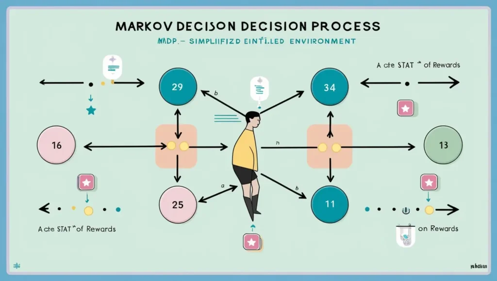
A visual representation of a Markov Decision Process (MDP) in a simplified environment. A central stylized agent moves through different states, represented by numbered or colored circles. Each state is connected by directional arrows indicating possible actions and transitions. Small icons like stars or tokens signify rewards near certain states, illustrating potential gains. The color palette includes light blues and pastel greens, with clear labels and annotations that visually explain the transition flow between states and actions in an MDP.

An MDP provides a mathematical framework for modeling decision-making where outcomes are partly random and partly under the control of the decision-maker.

States (S): All possible situations.
Actions (A): All possible actions.
Transition Function (T): Probability of moving from one state to another, given an action.
Reward Function (R): Immediate reward received after transitioning from one state to another due to an action.
Discount Factor (γ): A factor between 0 and 1 that reduces future rewards’ importance.

The Markov Property states that the future state depends only on the current state and action, not on the sequence of events that preceded it.

2.2 Policies and Value Functions

Policy (π): Defines the agent’s behavior, mapping states to actions.
State-Value Function (V(s)): Expected return starting from state s and following policy π.
Action-Value Function (Q(s, a)): Expected return starting from state s, taking action a, and thereafter following policy π.

2.3 The Bellman Equation

The Bellman Equation provides a recursive decomposition of the value function.

For the state-value function:

V(s)=∑aπ(a∣s)∑s′,rP(s′,r∣s,a)[r+γV(s′)]V(s) = \sum_{a} \pi(a|s) \sum_{s’, r} P(s’, r|s, a) [r + \gamma V(s’)]V(s)=∑aπ(a∣s)∑s′,rP(s′,r∣s,a)[r+γV(s′)]

This equation states that the value of a state is the expected return of the immediate reward plus the discounted value of the next state.

3. Core Reinforcement Learning Algorithms

3.1 Dynamic Programming

Dynamic Programming (DP) methods require a complete model of the environment and involve solving the Bellman equations directly.

Policy Evaluation: Calculates the value function for a given policy.
Policy Improvement: Improves the policy based on the value function.
Policy Iteration: Alternates between policy evaluation and policy improvement.
Value Iteration: Simultaneously updates the policy and value function.

3.2 Monte Carlo Methods

Monte Carlo methods learn directly from episodes of experience without requiring a model of the environment.

Episode-Based: Waits until the end of an episode to update value estimates.
Sample Averages: Uses the average of returns observed after visiting a state-action pair.
First-Visit and Every-Visit MC: Differ in how they handle multiple visits to the same state within an episode.

3.3 Temporal-Difference Learning

Temporal-Difference (TD) Learning combines ideas from DP and Monte Carlo methods.

Updates Estimates After Each Step: Unlike MC, which waits until the end of an episode.
TD(0) Algorithm: Updates the value of the current state based on the estimated value of the next state.

TD Update Rule:

V(st)←V(st)+α[rt+1+γV(st+1)−V(st)]V(s_t) \leftarrow V(s_t) + \alpha [r_{t+1} + \gamma V(s_{t+1}) – V(s_t)]V(st)←V(st)+α[rt+1+γV(st+1)−V(st)]

3.4 Q-Learning

Q-Learning is an off-policy TD control algorithm.

Goal: Learn the optimal action-value function Q∗(s,a)Q^*(s, a)Q∗(s,a).
Update Rule:

Q(st,at)←Q(st,at)+α[rt+1+γmax⁡aQ(st+1,a)−Q(st,at)]Q(s_t, a_t) \leftarrow Q(s_t, a_t) + \alpha [r_{t+1} + \gamma \max_{a} Q(s_{t+1}, a) – Q(s_t, a_t)]Q(st,at)←Q(st,at)+α[rt+1+γmaxaQ(st+1,a)−Q(st,at)]

Off-Policy: Learns the optimal policy independently of the agent’s actions.

3.5 SARSA

SARSA is an on-policy TD control algorithm.

Update Rule:

Q(st,at)←Q(st,at)+α[rt+1+γQ(st+1,at+1)−Q(st,at)]Q(s_t, a_t) \leftarrow Q(s_t, a_t) + \alpha [r_{t+1} + \gamma Q(s_{t+1}, a_{t+1}) – Q(s_t, a_t)]Q(st,at)←Q(st,at)+α[rt+1+γQ(st+1,at+1)−Q(st,at)]

On-Policy: Updates based on the action actually taken by the agent.

4. Deep Reinforcement Learning

4.1 Introduction to Deep RL

Deep Reinforcement Learning integrates deep neural networks with reinforcement learning architectures, enabling agents to make decisions from high-dimensional inputs like images.

4.2 Deep Q-Networks (DQN)

DQN combines Q-Learning with deep neural networks to approximate the action-value function.

Experience Replay: Stores transitions in a replay buffer to break correlations between sequential data.
Target Network: A separate network to stabilize learning by reducing oscillations.

DQN Loss Function:

L(θ)=E(s,a,r,s′)[(r+γmax⁡a′Qθ−(s′,a′)−Qθ(s,a))2]L(\theta) = \mathbb{E}_{(s,a,r,s’)} \left[ (r + \gamma \max_{a’} Q_{\theta^-}(s’, a’) – Q_\theta(s, a))^2 \right]L(θ)=E(s,a,r,s′)[(r+γmaxa′Qθ−(s′,a′)−Qθ(s,a))2]

4.3 Policy Gradient Methods

Instead of estimating value functions, policy gradient methods directly adjust the policy’s parameters.

Objective: Maximize the expected return.

Policy Gradient Theorem:

∇J(θ)=Eπθ[∇θlog⁡πθ(a∣s)Qπθ(s,a)]\nabla J(\theta) = \mathbb{E}_{\pi_\theta} \left[ \nabla_\theta \log \pi_\theta(a|s) Q^{\pi_\theta}(s, a) \right]∇J(θ)=Eπθ[∇θlogπθ(a∣s)Qπθ(s,a)]

Interested in the architecture that powers advanced agents? Read our tutorial on how to build a GAN from scratch, which also uses neural networks.

4.4 Actor-Critic Algorithms

Combines policy gradients (actor) and value function estimation (critic).

Actor: Updates the policy distribution in the direction suggested by the critic.
Critic: Estimates the value function.

Advantages:

Stability: Critic reduces variance in policy updates.
Efficiency: Actor leverages the critic’s feedback for more informed updates.

5. Advanced Topics

5.1 Exploration vs. Exploitation Trade-off

Exploration: Trying new actions to discover their effects.
Exploitation: Using known information to maximize rewards.

Strategies:

ε-Greedy Policy: Chooses a random action with probability ε, otherwise selects the best-known action.
Softmax Action Selection: Chooses actions probabilistically based on their estimated value.

5.2 Function Approximation

When state or action spaces are large, function approximation methods are used to estimate value functions or policies.

Linear Function Approximators
Non-linear Approximators (Neural Networks)

Challenges:

Bias and Variance Trade-off
Overfitting

5.3 Transfer Learning in RL

Applying knowledge learned in one task to improve learning in another related task.

Benefits: Reduces training time, improves performance.
Methods: Sharing parameters, initializing with pre-trained models.

5.4 Multi-Agent Reinforcement Learning

Involves multiple agents interacting within the same environment.

Cooperative Settings: Agents work together to achieve a common goal.
Competitive Settings: Agents compete against each other.

Complexities:

Non-Stationarity: The environment changes as other agents learn.
Scalability: Increases computational requirements.

6. Applications of Reinforcement Learning

6.1 Game Playing and Simulation

AlphaGo: Defeated human champions in Go using RL and deep neural networks.
Atari Games: DQN achieved human-level performance on various Atari games.

6.2 Robotics

Motion Control: RL enables robots to learn complex movements and adapt to new tasks.
Manipulation Tasks: Learning to grasp and manipulate objects in unstructured environments.

6.3 Finance

Trading Strategies: RL algorithms optimize buying and selling decisions.
Portfolio Management: Balancing assets to maximize returns and minimize risks.

Want to see how AI is already being used in real-world trading strategies? Check out our Python-based guide to AI in finance.

6.4 Healthcare

Treatment Policies: Personalizing treatment plans based on patient data.
Resource Allocation: Optimizing scheduling and allocation of medical resources.

6.5 Autonomous Vehicles

Navigation: Learning to navigate complex environments.
Decision-Making: Adapting to dynamic traffic conditions.

7. Challenges and Future Directions

7.1 Sample Efficiency

Problem: RL often requires a vast number of interactions with the environment.
Solutions: Model-based RL, transfer learning, and leveraging prior knowledge.

7.2 Safety and Ethics in RL

Safety Concerns: Unintended behaviors in critical systems.
Ethical Considerations: Ensuring fairness and preventing misuse.

Approaches:

Safe Exploration: Constraining the agent to avoid harmful actions.
Reward Shaping: Designing reward functions that align with desired outcomes.

7.3 Scaling RL to Real-World Problems

Complex Environments: Dealing with partial observability and uncertainty.
Computational Resources: High computational demands for training.

Advancements:

Distributed RL: Utilizing multiple agents and resources.
Hierarchical RL: Breaking down tasks into sub-tasks.

Learn how to address AI opacity and bias with our deep-dive on Explainable AI and transparency.

8. Implementing Reinforcement Learning in Python

8.1 Setting Up the Environment

Install the necessary libraries:

bash
pip install numpy gym tensorflow

8.2 A Simple RL Example with OpenAI Gym

We’ll implement a basic Q-Learning agent for the CartPole-v0 environment.

Step 1: Import Libraries

python
import gym
import numpy as np

Step 2: Initialize Environment and Q-Table

python
env = gym.make('CartPole-v0')
state_space = env.observation_space.shape[0]
action_space = env.action_space.n

q_table = np.zeros((state_space, action_space))

Note: CartPole has a continuous state space. For simplicity, we’ll discretize it.

Step 3: Discretize the State Space

python
def discretize_state(state):
    bins = np.array([-2.4, -1.2, 0.0, 1.2, 2.4])
    indices = np.digitize(state, bins)
    return tuple(indices)

Step 4: Set Hyperparameters

python
alpha = 0.1   # Learning rate
gamma = 0.99  # Discount factor
epsilon = 1.0 # Exploration rate
epsilon_min = 0.01
epsilon_decay = 0.995
episodes = 1000

Step 5: Training Loop

python
for episode in range(episodes):
    state = discretize_state(env.reset())
    done = False
    total_reward = 0
    
    while not done:
        # Epsilon-greedy action selection
        if np.random.rand() < epsilon:
            action = env.action_space.sample()
        else:
            action = np.argmax(q_table[state])
        
        # Take action
        next_state_raw, reward, done, _ = env.step(action)
        next_state = discretize_state(next_state_raw)
        
        # Update Q-Table
        old_value = q_table[state][action]
        next_max = np.max(q_table[next_state])
        
        new_value = old_value + alpha * (reward + gamma * next_max - old_value)
        q_table[state][action] = new_value
        
        state = next_state
        total_reward += reward
    
    # Decay epsilon
    if epsilon > epsilon_min:
        epsilon *= epsilon_decay
    
    if (episode + 1) % 100 == 0:
        print(f"Episode {episode + 1}/{episodes}, Total Reward: {total_reward}")

Step 6: Testing the Trained Agent

python
state = discretize_state(env.reset())
done = False
total_reward = 0

while not done:
    action = np.argmax(q_table[state])
    next_state_raw, reward, done, _ = env.step(action)
    next_state = discretize_state(next_state_raw)
    state = next_state
    total_reward += reward
    env.render()

env.close()
print(f"Total Reward: {total_reward}")

Disclaimer: This is a simplified example for illustrative purposes. In practice, handling continuous state spaces requires more sophisticated methods like function approximation.

9. Conclusion

Reinforcement Learning represents a cornerstone of modern AI, offering powerful tools for sequential decision-making problems. From foundational concepts like Markov Decision Processes to advanced algorithms in deep reinforcement learning, the field has evolved rapidly, finding applications across various industries.

As we continue to push the boundaries of what’s possible with AI, understanding reinforcement learning’s principles and challenges becomes increasingly important. Whether you’re developing autonomous systems, optimizing operations, or exploring theoretical aspects, RL provides a rich framework for innovation.

We encourage you to delve deeper, experiment with different algorithms, and contribute to this exciting domain. The future of AI is not just about intelligent systems but about systems that can learn and adapt through interaction—a vision that reinforcement learning embodies.

10. References

Sutton, R. S., & Barto, A. G. (2018). Reinforcement Learning: An Introduction. MIT Press.
Mnih, V., Kavukcuoglu, K., Silver, D., et al. (2015). Human-level control through deep reinforcement learning. Nature, 518(7540), 529-533.
Silver, D., Huang, A., Maddison, C. J., et al. (2016). Mastering the game of Go with deep neural networks and tree search. Nature, 529(7587), 484-489.
OpenAI Gym Documentation: https://gym.openai.com/docs/
Lillicrap, T. P., Hunt, J. J., Pritzel, A., et al. (2015). Continuous control with deep reinforcement learning. arXiv preprint arXiv:1509.02971.

About TechFlareAI

At TechFlareAI, we’re passionate about making artificial intelligence accessible and engaging for everyone. Our mission is to illuminate the path to innovation by providing in-depth guides, tutorials, and analyses on the latest trends and technologies in AI.

Join the Conversation

Have questions or insights about reinforcement learning? Share your thoughts in the comments below or join our community forum to engage with fellow AI enthusiasts!

Stay Connected

Subscribe to our newsletter to receive daily updates on AI trends, tutorials, and innovative projects delivered straight to your inbox.

Keywords: Reinforcement Learning, Artificial Intelligence, Machine Learning, Deep Learning, Markov Decision Processes, Q-Learning, Policy Gradients, Deep Q-Networks

Disclaimer: The information provided in this article is for educational purposes. Always consider additional research and professional advice for specific applications.